Randomisation Test Methods
A NONMEM User’s Perspective
Nick Holford 6 May 2001
How does one know alpha, the probability of rejecting the null hypothesis when in fact the null is true? For some analysis models and with small data sets alpha can be computed explicitly from the data e.g. Fisher’s exact test. For more complex analyses and for larger data sets it may either be theoretically impossible or computationally impractical to compute the exact probability. In this case the randomisation test can be used. It is a computational method relying upon randomisation to create a large number of data sets (replicates) that could have arisen under the null and then computing some statistic and examining its distribution. The empirical distribution of this statistic is then used to estimate alpha. A description of the basic idea of the randomisation test is provided by Lane [1] and a review of this and other computer intensive statistical methods can be found in Kelly [2].
The essence of the procedure is to define a covariate (e.g. treatment, sex, weight, etc.) in the original data set and to assign a covariate value randomly to each subject to create a new randomisation data set. For example, if the covariate was 1 for treatment with active drug and 0 with placebo then this would involve assigning 1 and 0 at random to each of the subjects in the data. Under the usual null hypothesis there should be no association between treatment and outcome when this randomised data set is analysed. The randomised data sets would each be in instance of how the data might have arisen under the null hypothesis. The distribution of a statistic which might reflect an effect of treatment on outcome will therefore reflect the distribution of this statistic when the null is true.
There are (at least) 3 methods that can be considered for the randomisation of the covariate:
- Sample from a parametric distribution for the covariate
- Sample with re-sampling from the covariate empirical distribution
- Sample by permutation of the covariate empirical distribution (no resampling)
Note that the first two methods could by chance lead to distributions of the covariate in the randomisation data set that were different from the original data e.g. if the original data had 50 subjects on active drug and 50 on placebo then these methods could easily produce data with, for example, 49 subjects on active and 51 on placebo.
Parametric Distribution
This requires a parametric model for the distribution of the covariate e.g. if the trial protocol called for randomisation equally between active treatment (1) and placebo (0) then given a uniform random number (uran) the randomised covariate value (randcov) can be determined as follows:
if (uran >= 0.5)
randcov=1
else
randcov=0
This method is analogous to a parametric bootstrap randomisation.
Empirical Distribution
The empirical distribution of the covariate is simply the covariate values in the data set. For simplicity it is assumed that each covariate does not change within each subject’s data. If the array containing the empirical distribution of covariates is COV and the number of subjects is nsub then a random sample from the empirical distribution can be determined as follows using uran:
isub=int(nsub*uran)+1
rancov=COV[isub]
This method is analogous to a non-parametric bootstrap randomisation.
Permutation
The permutation method ensures that the distribution of the covariates in the randomisation data set is identical to that seen in the original data set. This is done by randomly sampling from COV then deleting that value from COV so that the next sample is drawn from the remaining unsampled values. An algorithm for this is:
if (nsub>1) {
isub=int(nsub*uran)+1
rancov=COV[isub]
# remove COV[isub]
for
(i=isub; i<nsub; i++)
COV[i]=COV[i+1]
nsub--
} else
rancov=COV[1]
An Example
The theopd data set and NONMEM model describes the concentration effect relationship for theophylline effects on peak expiratory flow rate in patients with asthma. Theophylline concentrations were achieved in the course of a randomised concentration controlled trial[3, 4]. One possible covariate to explain the variability in the Emax parameter is sex. Models with (Figure 3) and without such a covariate effect were fit to the data. Using the FO estimation method the objective function difference was 5802.086-5798.270=3.816 and with FOCE the difference was 5801.331-5795.723=5.608.
The randomisation test was performed with 1000 replications using the three randomisation methods with both FO and FOCE NONMEM estimation options.
Table 1 Randomisation Test
Results. Observed DOBJ for FOCE=5.608
and for FO=3.816. Compaq Visual Fortran 6.6 /fltconsistency
/optimize:4 /fast
|
Estimation Method |
Randomization Method |
Successful Runs % |
P Chi-Square |
P Quantile |
DOBJ(0.05,1) |
|
FOCE |
Parametric |
99.7 |
0.018 |
0.028 |
4.506 |
|
|
Non-Parm |
99.2 |
0.018 |
0.033 |
4.570 |
|
|
Permutation |
99.4 |
0.018 |
0.024 |
4.163 |
|
FO |
Parametric |
99.7 |
0.051 |
0.073 |
4.407 |
|
|
Non-Parm |
99.7 |
0.051 |
0.080 |
4.741 |
|
|
Permutation |
98.7 |
0.051 |
0.065 |
4.115 |
The
results are shown in Table 1.
The P value from the chi-square distribution is shown for FO and FOCE based on
the observed difference in objective function between the null model and the
model including an effect of sex on Emax obtained from the original data set. A
P value was predicted from the empirical quantile of
the distribution of the difference between the null model objective function
(FO=5802.086, FOCE=5801.331) and the objective function obtained from each
randomisation replicate. In all cases the quantile P value is larger than that
predicted from the chi-square distribution.
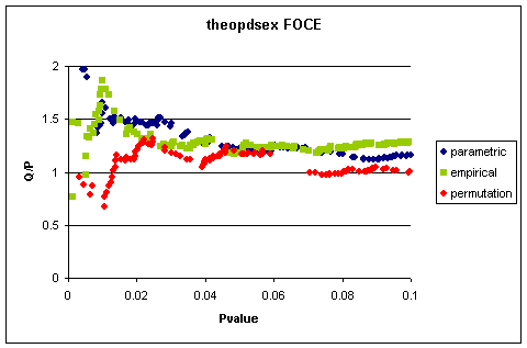
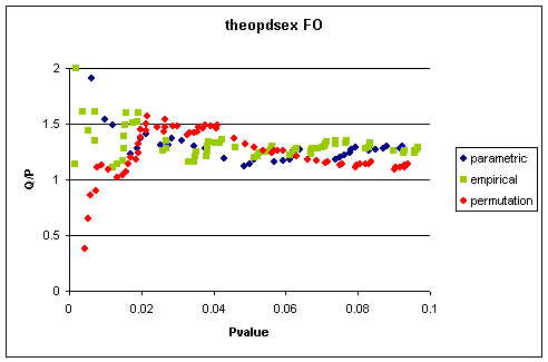
A
plot of the chi-square P value predicted from the objective function difference
for each replicate versus the empirical quantile for
that replicate is shown in Figure 1
and Figure 2.
This indicates that the empirical quantile estimate
is more or less the same for each randomisation method.
Conclusion
Each of the randomisation methods produces apparently similar results. There may be theoretical reasons to prefer one over another for particular applications. The permutation method is appealing because it guarantees that the covariate distribution is identical to the original data.
Figure 1 Quantile/Pvalue
Using FOCE Estimation

Figure 2 Quantile/Pvalue
Using FO Estimation

Figure 3 NM-TRAN Control Stream for Sex and Emax
$PROB THEOPHYLLINE PHARMACODYNAMICS STANDARD CONTROL STREAM
$DATA theopd.dat IGNORE #
$INPUT ID TIME THEO AGE WT SEX RACE DIAG DV
$ESTIM PRINT=0
$THETA (0,150.,) ; POPE0
$THETA (0,200.,) ; POPEMAX
$THETA (.001,10,) ; POPEC50
$THETA 1 ; EMSEX
$OMEGA 0.5 ; ETAE0
$OMEGA 0.5 ; ETAEMAX
$OMEGA 0.5 ; ETAEC50
$SIGMA 100 ; ERRSD
$PRED
IF (SEX.NE.1) THEN ;female
FSXM=THETA(4)
ELSE
FSXM=1
ENDIF
E0 =THETA(1)*EXP(ETA(1))
EMAX=FSXM*THETA(2)*EXP(ETA(2))
EC50=THETA(3)*EXP(ETA(3))
Y = E0 + EMAX*THEO/(THEO+EC50) + ERR(1)
References
1. Lane D. Randomization tests. In. HyperStat Online Textbook. ed: http://davidmlane.com/hyperstat/B163479.html; 2001.
2. Kelly P. Overview of Computer Intensive Statistical Inference Procedures. http://garnet.acns.fsu.edu/~pkelly/resampling.html. In.; 1999.
3. Holford N, Hashimoto Y, Sheiner LB. Time and theophylline concentration help explain the recovery of peak flow following acute airways obstruction. Clinical Pharmacokinetics 1993;25(6):506-15.
4. Holford NHG, Black P, Couch R, Kennedy J, Briant R. Theophylline target concentration in severe airways obstruction - 10 or 20 mg/L? Clinical Pharmacokinetics 1993;25(6):495-505.